In econometrics, Stata is a commonly used computer program for regression analysis. Below are some important commands and descriptions useful for doing regression analysis in Stata. R2 (R-squared)How much the linear regression explains the data, a value between 0-1. Also known as the coefficient of determination. If R-squared = 1, all observations are on a straight line, and the linear regression perfectly matches the data points. If R-squared = 0.4, the linear regression explains 40% of the variation in the data. If 0, it explains nothing. High R-squared is important if you want to use the model for prediction. Often high in general time series data, but does not necessarily teach us causation, so we should not only focus on it. Sometimes, a more specific data might generate a lower R^2, but we might learn something important on the way. R^2 = SSE/SST = 1 - SSR/SST 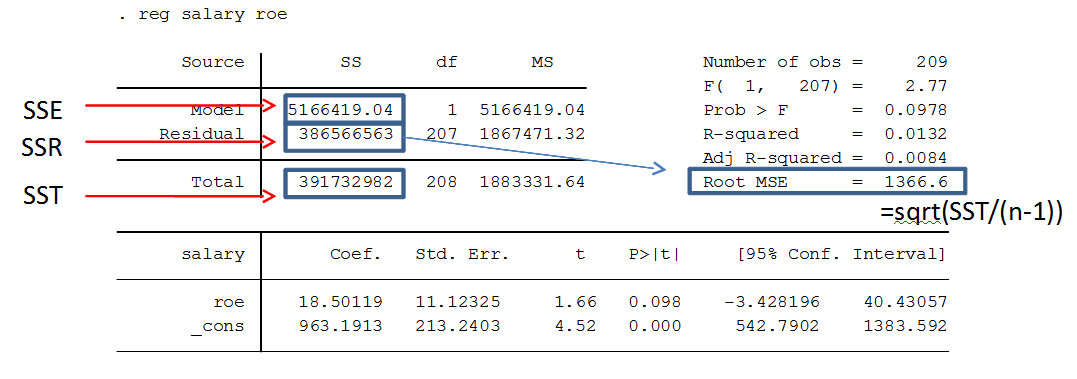 The R-squared is calculated from SSE, SSR and SST. 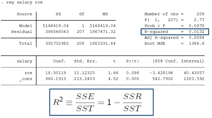 The formula for calculating R-squared. Definitions SST = Total Sum of Squares = SSE + SSR SSE = Explained Sum of Squares SSR = Residual Sum of Squares Adjusted R-squared Adjusted R-squared penalizes inclusion of more independent variables (since k increases). It can thus be a better measure when comparing results across different regression models. Normal R^2 = 1- (SSR/n) / (SST/n) Adjusted R^2 = 1- (SSR/n-k-1) / (SST/n-1) Natural logarithmThe natural logarithm (ln, or sometimes just log) is commonly used both on dependent variables and independent variables when we desire to transform the results into percent form. It is also used when we want to make our model more homoskedastic, by reducing the spread of values of the independent variables, making them more evenly distributed. The table below can be used as a guide for interpreting the results of logarithmic variables compared to normal ("level") variables.
The log-log model has the same form as elasticity (if you know Swedish, see Elasticitet). Thus, the log-log model is also known as the Constant Elasticity (CE) model. Exact percent When we use logarithm on the dependent variable, β*100 is just an approximation of the effect of a change in the independent variable. To get exact numbers, we must use the formula: 100 * (exp(β) - 1) Which can also be written: 100 * (e^β - 1) Where exp(β) is e to the power of the coefficient (β) we're looking at. Simple vs multiple regressionSimple linear regression (SLR): one independent variable Multiple linear regression (MLR): two+ independent variables 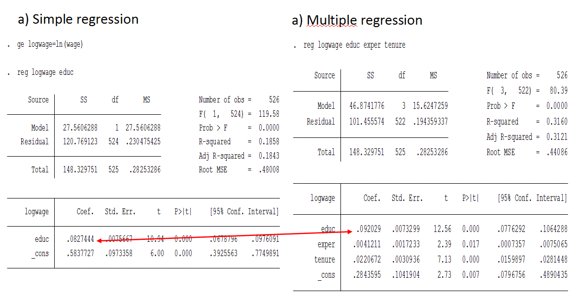 Simple vs multiple regression in Stata. Note that in the example above, the effect of education increases when we control for additional variables. This is because education is negatively correlated with experience and tenure, because people who study more enter the labor market later. However, all variables are positively correlated with wage. This means that by not controlling for the experience, we underestimate the effect of education of wages. Limited Dependent Variable (LDV)/Linear Probability Model (LPM)When the dependent variable (y) is a dummy/boolean variable (i.e. it can only have the value 0 or 1).If y can be 0 or 1, the expected value of y can be interpreted as the probability that y is equal to 1. Therefore, multiple linear regression model with binary dependent variable is called the linear probability model (LPM). It's often okay to use OLS even with LDV. Interaction termSometimes partial effects depend on another independent variable. In those cases it can be useful to include an interaction term, which is simply one independent variable times another.Example: price = B0 + B1 * sqrft + B2 * bedrooms + B3(sqrft * bedrooms) + B4 * bthrms + u Means that, the effect on price of adding more bedrooms depends on the size of the house: delta_price/delta_bedrooms = B2 + B3 * sqrtft It’s more expensive to add bedrooms to a small house than a large house. |
Regression analysis >
