This page describes some (but not yet all) basic terms and concepts in statistics and regression analysis. A random variable (or stochastic variable) is a variable that can take a random value from a set of possible values. Each value has an associated probability, which decides the likelihood of it being chosen. The two most common types of random variables are:
A probability distribution is a mathematical function describing the possible values of a random variable and their associated probabilities. The most common type of probability distribution is the normal distribution. The normal distribution (or bell curve) is the most common probability distribution. It has a distinct shape which makes it easy to remember. 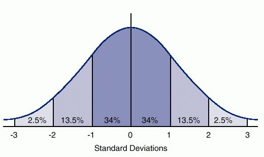 Normal distribution of values in a random variable. Example .svg.png) An example of an experiment of tossing two dice at the same time. The distribution of the sum of the two dice values would be normally distributed, as shown above. Source Some even say that any random variable will end up being normally distributed, given a large enough sample size (i.e. as long as the experiment is repeated enough times). This is known as the central limit theorem (CLT). Expected value (population mean)The expected value or population mean (μ) is the average value we would expect to find from a random variable if we repeated an experiment an infinite number of times. In theory, the result is the same as the average or arithmetic mean value, i.e. the sum of all values divided by the number of values, although it's calculated a bit differently. Definition The expected value is the sum of all possible values for a random variable, each value multiplied by its probability of occurrence. E[X] = x1p1 + x2p2 + ... + xnpn Where: E[X] is the expected value of random variable X x1 to xn represents all the possible values that X can take. p1 to pn is the probability of this value occurring Example The expected value for rolling a dice is: E[X] = 1*1/6 + 2*1/6 + 3*1/6 + 4*1/6 + 5*1/6 + 6*1/6 = 3.5 There's a 1/6 chance that the dice lands on each side. If we role the dice an infinite number of times, the average value should be 3.5. Definition The variance of a random variable is the expected value of the squared deviation from the mean: Var(X) = E[(X - μ)^2] Where: Var(X) is the variance of the random variable X μ is the mean, which is the same as the expected value of X, i.e. μ = E[X] Example (simplified) Let's say we have eight data points with the values 2+4+4+4+5+5+7+9. The mean (μ) of these values are: μ = (2+4+4+4+5+5+7+9) / 8 = 5 For each value, we take its deviation from the mean and square it: (2-5)^2 = 9 (4-5)^2 = 1 (4-5)^2 = 1 (4-5)^2 = 1 (5-5)^2 = 0 (5-5)^2 = 0 (7-5)^2 = 4 (9-5)^2 = 16 We then get the mean (expected value) of these to get the variance: Var(X) = (9+1+1+1+0+0+4+16) / 8 = 2 The standard deviation (σ) is the square root of the variance: σ = sqrt(2) = 1.41421356237 This means that the variance of X is the standard deviation (σ) of X squared: Var(X) = σ^2 Standard deviationThe standard deviation (σ) is another way of expressing the variance, calculated as the square root of the variance.Definition The square root of the variance: σ = sqrt(Var(X)) Or you could write: σ^2 = Var(X) σ is the standard deviation of the random variable X Var(X) is the variance of X Covariance is a measure of the relationship between two random variables. How much the two variables vary together, and in what direction. The covariance is positive when the variables move in the same direction, and negative when they move in opposite directions. Zero covariance means there is no linear relationship between them. Covariance is measured in the same units as the variables, making it hard to compare between variables. Correlation fixes this by standardizing the values, giving us a fixed range of -1 to 1. Definition Cov[X,Y] = E[(X - E[X]) * (Y - E[Y])] = E[XY] - E[X] * E[Y] If we take the covariance of a variable with itself, this simply equals its variance: Cov[X,X] = Var[X] CorrelationCorrelation is a measure of the relationship between two random variables. How much the two variables vary together, and in what direction. It's the same as the covariance, except it uses a standardized range of values between -1 to 1 while covariance is measured in the same unit as the variables. A value of 1 means a perfect positive relationship, -1 a perfect negative relationship, and 0 means no relationship at all. Note that correlation does not imply causation. Just because there is a statistical relationship between two things does not mean that one causes the other, only that they seem to occur at roughly the same time. This also holds for covariance. Definition Corr(X,Y) = Cov[X,Y] / sqrt(Var[X] * Var[Y]) There are different types of data, which require different regression methods:
|
Regression analysis >
