To ensure that our linear regression model can be trusted we want it to adhere to certain standards. These standards are defined as assumptions, and the closer our model is to these ideal assumptions, the better our model is.
The assumptions vary slightly depending on what type of regression we're dealing with:
SLR: Simple linear regression (one independent variable)
MLR: Multiple linear regression (two+ independent variables)
TS: Time series regression
The assumptions below are collectively known as the Classical Linear Model (CLM) assumption.
Innehåll
- 1 Linearity & unbiasedness
- 1.1 Linear in parameters (SLR.1, MLR.1, TS.1)
- 1.2 Random sampling (SLR.2, MLR.2)
- 1.3 Sample variation & No perfect collinearity(SLR.3, MLR.3, TS.2)
- 1.4 Zero conditional mean/No omitted variables(SLR.4, MLR.4, TS.3)
- 2 Best Linear Unbiased Estimator (BLUE)
- 2.1 Homoskedasticity (SLR.5, MLR.5, TS.4)
- 2.2 No serial correlation/autocorrelation(TS.5)
- 3 Normality
- 3.1 Normality(MLR.6, TS.6)
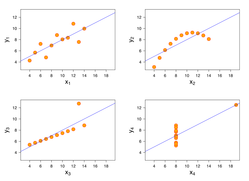
Although it's important test your model mathematically, you should always analyse it visually as well, as some things are hard to spot mathematically, but easy to spot by eye.
Read more
Under the following four assumptions, the OLS estimator is unbiased, meaning our model can be trusted not to output biased (i.e. misleading) results. It is also linear in parameters, so it's sometimes called the "Linear Unbiased Estimator" (LUE).
Formally, an estimator is unbiased if our expected predicted coefficients (βhat) are equal to the actual coefficients (β):
E(βhat) = β
Linear in parameters
(SLR.1, MLR.1, TS.1)
The model must be linear in its parameters. The parameters are the coefficients on the independent variables (often marked as β). In other words, the model must have linear coefficients. For example: y = β0 + β1 * x1 + u is valid, while y = β1 + β1^2 * x1 + u is not, because the coefficient β1^2 is not linear.
This assumption is why we call it "linear" regression. Linear regression simply means it must be linear in parameters (coefficients). Although the coefficients must be linear, the dependent and independent variables must not, which allows us to model nonlinear relationships, for example by including a squared variable.
Random sampling
(SLR.2, MLR.2)
The model must have randomly selected values, meaning that the values themselves of an independent variable should not be corelated.
In time series regression, this assumption is omitted, as it's captured in other assumptions.
Sample variation & No perfect collinearity
(SLR.3, MLR.3, TS.2)
We must have at least some variation in our sample values, meaning that all values cannot be the same.
In multi-variable regression (MLR), we must also have no perfect linear relationship between independent variables. If an independent variable has a perfect linear relationship with another independent variables, we say that the model suffers from perfect collinearity, and it cannot be estimated by OLS. This doesn't mean that two independent variables cannot be correlated, just that they cannot be perfectly linearly correlated.
One of the most common examples of perfect collinearity are two measures of income, one in dollar and one in thousands of dollars. One of these is redundant and should be removed, as it violates this assumption. Note that this only holds for linear relationship, so for example including a squared version of an independent variable is still okay.
Zero conditional mean/No omitted variables
(SLR.4, MLR.4, TS.3)
There are no omitted variables that we have been left out, that correlates with one of our independent variables. In other words, there is no correlation between the error term (that captures all external factors and omitted variables) and our independent variables, i.e. the mean of the error term conditioned on each independent variable is zero (see Definition).
If this was the case, we would have an omitted-variable bias (OVB), as we have left out an important causal factor. This means we might draw incorrect conclusions on causation, by over- or underestimation the effect of our included variables.
This is one of the most important and common errors in regression analysis in practice, and is also known as the correlation/causation problem, "correlation does not imply causation" or simply "jumping to conclusions". In short, we want to find the root causes and direct effects rather than just analysing indirect relationships.
Non-zero conditional mean might also be caused by misspecification and measurement errors. For example, by forgetting to include a quadratic variable to account for non-linear effects of an independent variable.
The solution is to either add the omitted variable to the model as an extra independent variable, or use an instrumental variable (IV) estimation.
When this assumption holds, we say that the independent variables are exogenous, as they do not depend on any of the other variables within the model (including the error term). If a variable depends on at least one other variable within the model, it's said to be endogenous,
Example 1
Let's say we analyse the effect of education on crime rate. Crime is our dependent variable and level of education our independent variable. We see that increased education is related with less crime, and might be tempted to draw the conclusion that education reduces the likelihood of committing a crime. However, let's say that an omitted variable, drug abuse, is also related with education. People with less education are more likely to use drugs, and people on drugs are more likely to commit crime. If this is the case, we have an omitted-variable bias. Education is overestimated as it also accounts for drug use. In general, drawing incorrect conclusions might mean we focus on the wrong things, fighting symptoms rather than root causes.
Example 2
Let's say we analyse an IQ score of Africans. IQ score is our dependent variable, African is our independent variable. We might come to the conclusion that Africans have less IQ than others. However, as we did not include any variable on level of education, we likely have an omitted-variable bias. Education likely has a negative correlation with being an African, meaning that you're more likely to have a low level of education if you're African. By omitting level of education, we overestimate the effect of being African, and risk drawing incorrect conclusions. It's your level of education and other similar factors that determine your IQ score, rather than what country you were born in.
Definition
The mean (expected value) of the error term (u), given any value of the independent variable (x), must be equal to zero:
E[u|x] = 0
Definition MLR
For multiple regression (MLR) with many independent variables, we simply say that the error term (u) must be uncorrelated with all independent variables:
E[u|x1, x1, ..., xk) = 0
Best Linear Unbiased Estimator (BLUE)
The next step is to get an unbiased variance. We do this by adding the assumption of homoskedasticity, and for time series we must also add no serial correlation. If these assumptions hold, the OLS estimator is now also said to be "Best", making it the “Best Linear Unbiased Estimator” (BLUE). In short, this means that there is no better estimator than the OLS for this particular model.
All of the assumptions 1-5 are collectively known as the Gauss-Markov assumptions.
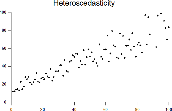
Homoskedasticity
(SLR.5, MLR.5, TS.4)
Constant variance across the error term. Even distribution of values, i.e. the same distance between data points and the regression line.
In other words, the error term u has the same variance given any value of the independent variables.
The opposite is called heteroskedasticity and is problematic because it risks overestimating the strength of relationships.
Transforming values to their natural logarithms generally helps reduce variation and make values more evenly distributed.
No serial correlation/autocorrelation
(TS.5)
The model must have no serial correlation (also known as autocorrelation) in the error terms.
Serial correlation or autocorrelation in the error terms means that the error terms are related across time. In other words, there is a pattern across the error terms. This indicates that the error terms are not independently distributed across the observations and are not strictly random.
The problem of serial correlation in the error terms is that estimated standard errors will be wrong. For example, with a positive serial correlation in the error terms, standard errors will be too low, which means you will tend to reject the null hypothesis too often.
Definition
Conditional on X, the error term (u) in two different time periods are uncorrelated, for all t different from s: Corr[u_t, u_s|X] = 0
After adding one final assumption, we have a complete set of assumptions that are collectively known as the Classical Linear Model (CLM) assumption.
The error term u is independent of the independent variables and is normally distributed with zero mean and variance σ2: u ~ Normal(0, σ2).